


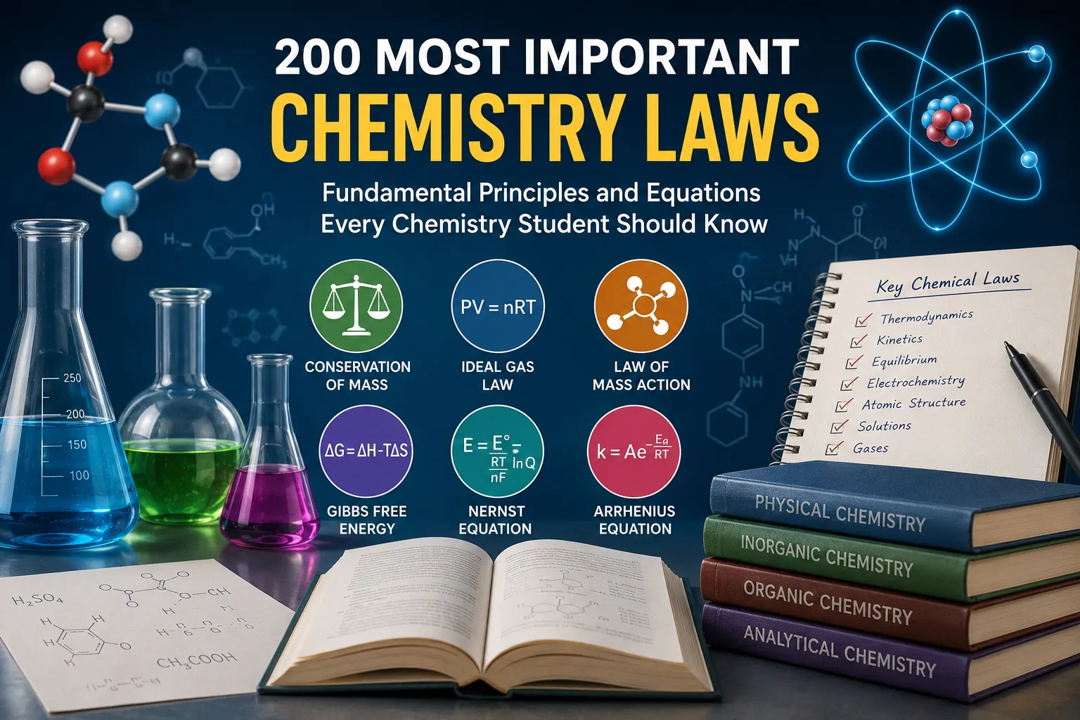
Chemistry is one of the fundamental branches of science that focuses on the composition, structure, properties, and transformations of matter.
It helps us understand how substances interact with one another and explains many of the processes that occur around us, from everyday chemical reactions to complex processes in living organisms, industry, medicine, and the environment.
Chemistry is closely connected to other scientific disciplines, including physics, biology, geology, and materials science, making it an essential field of study in both education and scientific research.
The study of chemistry involves many important laws, principles, equations, and mathematical relationships that help explain and predict chemical behavior.
These laws are essential for understanding topics such as chemical reactions, gases, solutions, thermodynamics, equilibrium, kinetics, electrochemistry, atomic structure, and molecular interactions.
Whether you are a high school student, a university student, a chemistry teacher, or simply interested in learning chemistry, knowing these fundamental laws can make many chemical concepts easier to understand and apply.
In this article, we have compiled 200 of the most famous and widely used laws and equations in chemistry.
The list covers different areas of chemistry and is designed to be useful for students at different educational levels, particularly high school and university students.
200 Most Important Chemistry Laws and Equations
Below is a comprehensive list of 200 important and widely used chemistry laws, principles, equations, and relationships.
It includes fundamental concepts that are commonly studied by students in both secondary and higher education and can serve as a useful reference for studying, reviewing, and solving chemistry problems.
| # | Law / Equation | Formula | Main Use |
|---|---|---|---|
| 1 | Law of Conservation of Mass | Mass of reactants = Mass of products | Conservation of matter in chemical reactions |
| 2 | Law of Definite Proportions | Fixed mass ratio of elements | Determines composition of compounds |
| 3 | Law of Multiple Proportions | Simple whole-number ratios | Compares different compounds of the same elements |
| 4 | Law of Reciprocal Proportions | Equivalent combining ratios | Relates combining proportions of elements |
| 5 | Gay-Lussac’s Law of Combining Volumes | V₁:V₂ = simple whole-number ratio | Relates gas volumes in reactions |
| 6 | Avogadro’s Law | V ∝ n | Relates gas volume to amount of gas |
| 7 | Boyle’s Law | P₁V₁ = P₂V₂ | Pressure-volume relationship |
| 8 | Charles’s Law | V₁/T₁ = V₂/T₂ | Temperature-volume relationship |
| 9 | Gay-Lussac’s Pressure Law | P₁/T₁ = P₂/T₂ | Temperature-pressure relationship |
| 10 | Combined Gas Law | P₁V₁/T₁ = P₂V₂/T₂ | Combines gas relationships |
| 11 | Ideal Gas Law | PV = nRT | Calculates gas properties |
| 12 | Dalton’s Law of Partial Pressures | Ptotal = ΣPᵢ | Total pressure of gas mixtures |
| 13 | Graham’s Law of Effusion | r₁/r₂ = √(M₂/M₁) | Compares gas effusion rates |
| 14 | Henry’s Law | C = kHP | Gas solubility in liquids |
| 15 | Amontons’s Law | P/T = constant | Pressure-temperature relationship |
| 16 | van der Waals Equation | (P + an²/V²)(V − nb) = nRT | Describes real gases |
| 17 | Compressibility Factor | Z = PV/nRT | Measures deviation from ideal gas behavior |
| 18 | Boyle Temperature Relation | B(TB) = 0 | Describes gas behavior near ideality |
| 19 | Critical Point Relation | Tc, Pc, Vc | Describes critical state of substances |
| 20 | Root Mean Square Speed | uᵣₘₛ = √(3RT/M) | Calculates molecular gas speed |
| 21 | Average Molecular Speed | uavg = √(8RT/πM) | Calculates average molecular speed |
| 22 | Most Probable Speed | ump = √(2RT/M) | Determines most probable molecular speed |
| 23 | Kinetic Molecular Energy | KEavg = 3RT/2 | Relates temperature to molecular motion |
| 24 | Maxwell-Boltzmann Distribution | f(v) distribution | Describes molecular speed distribution |
| 25 | Graham’s Diffusion Relation | Rate ∝ 1/√M | Compares diffusion rates |
| 26 | Raoult’s Law | Pᵢ = XᵢPᵢ° | Vapor pressure of solutions |
| 27 | Modified Raoult’s Law | Pᵢ = γᵢXᵢPᵢ° | Non-ideal solution behavior |
| 28 | Dalton’s Law for Vapor Mixtures | Ptotal = ΣPᵢ | Vapor mixture pressure |
| 29 | Clausius-Clapeyron Equation | ln(P₂/P₁) = −ΔHvap/R(1/T₂ − 1/T₁) | Vapor pressure vs temperature |
| 30 | Trouton’s Rule | ΔSvap ≈ 85–88 J mol⁻¹ K⁻¹ | Estimates entropy of vaporization |
| 31 | Gibbs Phase Rule | F = C − P + 2 | Determines degrees of freedom |
| 32 | Lever Rule | Fraction = opposite segment/total | Determines phase composition |
| 33 | Nernst Distribution Law | C₁/C₂ = constant | Solute distribution between phases |
| 34 | Partition Coefficient | K = Corganic/Caqueous | Measures distribution between solvents |
| 35 | Henry’s Law for Volatility | P = kHx | Relates dissolved gas to partial pressure |
| 36 | Molarity Equation | M = n/V | Calculates solution concentration |
| 37 | Molality Equation | m = n/kg solvent | Concentration independent of temperature |
| 38 | Mole Fraction Equation | Xᵢ = nᵢ/Σn | Composition of mixtures |
| 39 | Normality Equation | N = equivalents/L | Equivalent-based concentration |
| 40 | Mass Percent | % mass = mass solute/mass solution ×100 | Solution composition |
| 41 | Volume Percent | % volume = volume solute/volume solution ×100 | Liquid mixture composition |
| 42 | Molarity-Dilution Equation | M₁V₁ = M₂V₂ | Dilution calculations |
| 43 | Concentration-Mass Equation | C = m/V | Concentration calculations |
| 44 | Mole Equation | n = m/M | Converts mass to moles |
| 45 | Avogadro Constant Relation | N = nNA | Number of particles |
| 46 | Avogadro Constant | NA = 6.02214076 × 10²³ mol⁻¹ | Converts moles to particles |
| 47 | Molar Volume of Ideal Gas | Vₘ = RT/P | Gas volume per mole |
| 48 | Density of an Ideal Gas | d = PM/RT | Gas density |
| 49 | Relative Density of Gas | d₁/d₂ = M₁/M₂ | Compares gas densities |
| 50 | Percent Yield Equation | % yield = actual/theoretical ×100 | Reaction efficiency |
| 51 | Percent Error | % error = | experimental−accepted |
| 52 | Percent Composition | % element = mass element/mass compound ×100 | Determines elemental composition |
| 53 | Empirical Formula Relation | Molecular formula = empirical formula × n | Determines molecular formula |
| 54 | Degree of Unsaturation | DBE = (2C + 2 + N − H − X)/2 | Determines molecular unsaturation |
| 55 | Atom Economy | %AE = desired product mass/total reactant mass ×100 | Measures synthetic efficiency |
| 56 | Stoichiometric Ratio | nA/a = nB/b | Quantitative reaction calculations |
| 57 | Limiting Reagent Relation | Product determined by limiting reactant | Identifies limiting reagent |
| 58 | Equivalent Weight Equation | Eq. wt. = molar mass/n-factor | Equivalent calculations |
| 59 | Normality-Molarity Relation | N = M × n-factor | Converts molarity to normality |
| 60 | Faraday’s Law of Electrolysis | m = ZIt | Electrolysis calculations |
| 61 | Faraday’s First Law | m ∝ Q | Mass deposited during electrolysis |
| 62 | Faraday’s Second Law | m₁/m₂ = E₁/E₂ | Compares electrochemical deposition |
| 63 | Charge Equation | Q = It | Electrical charge calculation |
| 64 | Faraday Constant | F ≈ 96485 C mol⁻¹ | Electrochemical calculations |
| 65 | Coulomb’s Law | F = kq₁q₂/r² | Electrostatic force |
| 66 | Electric Potential Energy | U = kq₁q₂/r | Charge interaction energy |
| 67 | Born Equation | ΔGsolv ≈ −kq²/(2r)(1−1/ε) | Solvation energy estimation |
| 68 | Debye-Hückel Limiting Law | log γᵢ = −Azᵢ²√I | Activity coefficients |
| 69 | Ionic Strength Equation | I = ½Σcᵢzᵢ² | Measures ionic environment |
| 70 | Kohlrausch’s Law | Λ°m = Σνᵢλ°ᵢ | Limiting ionic conductivity |
| 71 | Ohm’s Law | V = IR | Electrical resistance |
| 72 | Conductance Equation | G = 1/R | Electrical conductance |
| 73 | Conductivity Equation | κ = G(l/A) | Solution conductivity |
| 74 | Molar Conductivity | Λm = κ×1000/C | Conductivity per mole |
| 75 | Arrhenius Equation | k = Ae⁻ᴱᵃ/ᴿᵀ | Temperature dependence of reaction rate |
| 76 | Linear Arrhenius Equation | ln k = ln A − Ea/RT | Determines activation energy |
| 77 | Two-Temperature Arrhenius Equation | ln(k₂/k₁)=−Ea/R(1/T₂−1/T₁) | Compares rate constants |
| 78 | Collision Theory | k ∝ collision frequency × orientation | Explains reaction rates |
| 79 | Transition State Theory | k = κ(kBT/h)e⁻ΔG‡/RT | Calculates reaction rates |
| 80 | Eyring Equation | k = (kBT/h)e⁻ΔG‡/RT | Transition-state kinetics |
| 81 | Gibbs Activation Energy | ΔG‡ = ΔH‡ − TΔS‡ | Reaction activation analysis |
| 82 | van’t Hoff Equation | ln(K₂/K₁)=−ΔH°/R(1/T₂−1/T₁) | Temperature effect on equilibrium |
| 83 | Law of Mass Action | K = products/reactants | Chemical equilibrium |
| 84 | Equilibrium Constant | Kc = [products]/[reactants] | Equilibrium calculations |
| 85 | Kp Equation | Kp = Kc(RT)Δn | Gas equilibrium |
| 86 | Reaction Quotient | Q = products/reactants | Predicts reaction direction |
| 87 | Le Chatelier’s Principle | System shifts to oppose change | Predicts equilibrium shifts |
| 88 | Equilibrium Relation | ΔG° = −RT ln K | Relates Gibbs energy to equilibrium |
| 89 | Gibbs Reaction Energy | ΔG = ΔG° + RT ln Q | Determines reaction spontaneity |
| 90 | Equilibrium Condition | ΔG = 0 | Defines equilibrium |
| 91 | Thermodynamic Equilibrium Relation | K = e⁻ΔG°/RT | Calculates equilibrium constant |
| 92 | Hess’s Law | ΔHrxn = ΣΔHsteps | Calculates reaction enthalpy |
| 93 | First Law of Thermodynamics | ΔU = q + w | Energy conservation |
| 94 | Enthalpy Equation | H = U + PV | Defines enthalpy |
| 95 | Reaction Enthalpy | ΔH = ΣHproducts − ΣHreactants | Heat of reaction |
| 96 | Kirchhoff’s Law | d(ΔH)/dT = ΔCp | Temperature correction of enthalpy |
| 97 | Bond Enthalpy Equation | ΔH ≈ ΣD(bonds broken) − ΣD(bonds formed) | Estimates reaction enthalpy |
| 98 | Heat Equation | q = mcΔT | Heat calculations |
| 99 | Molar Heat Equation | q = nCmΔT | Heat per mole |
| 100 | Calorimetry Equation | qsystem + qsurroundings = 0 | Calorimetric calculations |
| 101 | Second Law of Thermodynamics | ΔSuniverse ≥ 0 | Determines entropy direction |
| 102 | Entropy Change Equation | ΔS = qrev/T | Calculates entropy change |
| 103 | Standard Entropy Change | ΔS° = ΣS°products − ΣS°reactants | Reaction entropy |
| 104 | Third Law of Thermodynamics | S = 0 at 0 K for perfect crystal | Defines absolute entropy |
| 105 | Gibbs Free Energy Equation | ΔG = ΔH − TΔS | Predicts spontaneity |
| 106 | Standard Gibbs Energy | ΔG° = ΣG°products − ΣG°reactants | Reaction spontaneity |
| 107 | Helmholtz Free Energy | A = U − TS | Thermodynamic spontaneity at constant T,V |
| 108 | Gibbs-Helmholtz Equation | ∂(ΔG/T)/∂T = −ΔH/T² | Temperature dependence of free energy |
| 109 | Maxwell Relation 1 | (∂S/∂V)T = (∂P/∂T)V | Thermodynamic property relationships |
| 110 | Maxwell Relation 2 | (∂S/∂P)T = −(∂V/∂T)P | Thermodynamic calculations |
| 111 | Maxwell Relation 3 | (∂T/∂V)S = −(∂P/∂S)V | Thermodynamic relationships |
| 112 | Maxwell Relation 4 | (∂T/∂P)S = (∂V/∂S)P | Thermodynamic relationships |
| 113 | Joule-Thomson Coefficient | μJT = (∂T/∂P)H | Gas cooling/heating |
| 114 | Joule-Thomson Relation | μJT = [T(∂V/∂T)P − V]/Cp | Calculates throttling behavior |
| 115 | Gibbs-Duhem Equation | SdT − VdP + Σnᵢdμᵢ = 0 | Multicomponent thermodynamics |
| 116 | Chemical Potential | μᵢ = μᵢ° + RT ln aᵢ | Chemical equilibrium |
| 117 | Ideal Solution Chemical Potential | μᵢ = μᵢ° + RT ln Xᵢ | Ideal solution behavior |
| 118 | Clapeyron Equation | dP/dT = ΔHtrans/(TΔVtrans) | Phase transition slope |
| 119 | Fusion Clapeyron Relation | dP/dT = ΔHfus/(TΔVfus) | Solid-liquid equilibrium |
| 120 | Vaporization Clapeyron Relation | dP/dT = ΔHvap/(TΔVvap) | Liquid-vapor equilibrium |
| 121 | Beer-Lambert Law | A = εbc | Absorption spectroscopy |
| 122 | Lambert Law | A ∝ b | Effect of path length on absorbance |
| 123 | Beer Law | A ∝ c | Effect of concentration on absorbance |
| 124 | Absorbance-Transmittance Relation | A = −log T | Spectroscopic calculations |
| 125 | Transmittance Equation | T = I/I₀ | Light transmission |
| 126 | Molar Absorptivity Relation | ε = A/bc | Determines molar absorptivity |
| 127 | Bragg’s Law | nλ = 2d sinθ | X-ray diffraction |
| 128 | Scherrer Equation | D = Kλ/(βcosθ) | Estimates crystallite size |
| 129 | de Broglie Equation | λ = h/p | Matter-wave wavelength |
| 130 | Planck-Einstein Relation | E = hν | Photon energy |
| 131 | Wavelength-Frequency Relation | c = λν | Relates wavelength and frequency |
| 132 | Photon Energy-Wavelength Relation | E = hc/λ | Calculates photon energy |
| 133 | Heisenberg Uncertainty Principle | ΔxΔp ≥ ħ/2 | Quantum measurement limits |
| 134 | Bohr Energy Equation | En = −13.6Z²/n² eV | Hydrogen-like atomic energies |
| 135 | Bohr Radius | rₙ = a₀n²/Z | Atomic orbital radius |
| 136 | Rydberg Equation | 1/λ = RZ²(1/n₁² − 1/n₂²) | Atomic spectra |
| 137 | Rydberg Energy Equation | ΔE = −hcRZ²(1/n₂²−1/n₁²) | Electronic transitions |
| 138 | Schrödinger Equation | Ĥψ = Eψ | Quantum mechanical systems |
| 139 | Time-Independent Schrödinger Equation | Ĥψ = Eψ | Atomic and molecular energy states |
| 140 | Born Interpretation | ψ | |
| 141 | Pauli Exclusion Principle | No two electrons share all four quantum numbers | Electron configuration |
| 142 | Hund’s Rule | Electrons occupy degenerate orbitals singly first | Electron configuration |
| 143 | Aufbau Principle | Orbitals fill from lower to higher energy | Electron configuration |
| 144 | Heisenberg Relation | ΔEΔt ≥ ħ/2 | Energy-time uncertainty |
| 145 | Compton Equation | Δλ = h(1−cosθ)/(mc) | Photon-electron scattering |
| 146 | Bohr Frequency Condition | ΔE = hν | Electronic transitions |
| 147 | Hydrogenic Ionization Energy | IE = 13.6Z²/n² eV | Ionization of hydrogen-like ions |
| 148 | Moseley’s Law | √ν = a(Z−b) | Relates X-ray frequency to atomic number |
| 149 | Hund’s Maximum Multiplicity Rule | Maximum unpaired electrons | Predicts electron arrangements |
| 150 | Effective Nuclear Charge | Zeff = Z − σ | Estimates nuclear attraction |
| 151 | Coulombic Atomic Energy | E ∝ −Zeff²/n² | Approximate atomic energy |
| 152 | Heitler-London Concept | ψ = ψAψB combinations | Chemical bonding description |
| 153 | Valence Bond Principle | Orbital overlap forms bonds | Covalent bonding |
| 154 | Molecular Orbital Principle | Atomic orbitals combine into MOs | Molecular electronic structure |
| 155 | Bond Order Equation | BO = ½(Nbonding − Nantibonding) | Bond strength and stability |
| 156 | Formal Charge Equation | FC = V − (N + B/2) | Lewis structure analysis |
| 157 | Dipole Moment | μ = qr | Molecular polarity |
| 158 | Polarizability Relation | α = induced dipole/electric field | Molecular response to fields |
| 159 | London Dispersion Energy | E ∝ −α₁α₂/r⁶ | Intermolecular attraction |
| 160 | Debye Interaction | E ∝ −μ²α/r⁶ | Dipole-induced dipole forces |
| 161 | Keesom Interaction | E ∝ −μ₁²μ₂²/(T r⁶) | Dipole-dipole interactions |
| 162 | van der Waals Attraction | E ∝ −1/r⁶ | Intermolecular forces |
| 163 | Born Repulsion | E ∝ 1/rⁿ | Short-range repulsion |
| 164 | Lennard-Jones Potential | V = 4ε[(σ/r)¹² − (σ/r)⁶] | Molecular interaction potential |
| 165 | Fick’s First Law | J = −D(dc/dx) | Diffusion at steady state |
| 166 | Fick’s Second Law | ∂c/∂t = D∂²c/∂x² | Time-dependent diffusion |
| 167 | Stokes’ Law | F = 6πηrv | Motion of particles in fluids |
| 168 | Einstein-Stokes Equation | D = kBT/(6πηr) | Diffusion coefficient |
| 169 | Nernst-Einstein Equation | σ = Σcᵢzᵢ²F²Dᵢ/RT | Ionic conductivity |
| 170 | Stokes-Einstein Relation | D = kBT/(6πηr) | Diffusion in liquids |
| 171 | Graham’s Law | Rate ∝ 1/√M | Gas diffusion and effusion |
| 172 | Raoult’s Law for Nonvolatile Solute | ΔP = XsoluteP° | Vapor-pressure lowering |
| 173 | Colligative Property Relation | Property ∝ number of particles | Solution properties |
| 174 | Boiling Point Elevation | ΔTb = Kb m | Boiling point changes |
| 175 | Freezing Point Depression | ΔTf = Kf m | Freezing point changes |
| 176 | Osmotic Pressure Law | π = MRT | Osmotic pressure |
| 177 | van’t Hoff Factor | i = observed particles/expected particles | Electrolyte effects |
| 178 | Modified Osmotic Pressure | π = iMRT | Electrolyte solutions |
| 179 | Boyle-van’t Hoff Relation | πV = nRT | Osmotic behavior |
| 180 | Henderson-Hasselbalch Equation | pH = pKa + log([A⁻]/[HA]) | Buffer pH |
| 181 | Acid Dissociation Constant | Ka = [H⁺][A⁻]/[HA] | Acid strength |
| 182 | Base Dissociation Constant | Kb = [BH⁺][OH⁻]/[B] | Base strength |
| 183 | Water Ionization Constant | Kw = [H⁺][OH⁻] | Aqueous equilibrium |
| 184 | pH Equation | pH = −log[H⁺] | Acidity measurement |
| 185 | pOH Equation | pOH = −log[OH⁻] | Basicity measurement |
| 186 | pH-pOH Relation | pH + pOH = 14 at 25°C | Relates acidity and basicity |
| 187 | Ka-Kb Relation | KaKb = Kw | Conjugate acid-base systems |
| 188 | Ostwald Dilution Law | Ka = Cα²/(1−α) | Weak electrolyte dissociation |
| 189 | Buffer Equation | [H⁺] = Ka([HA]/[A⁻]) | Buffer calculations |
| 190 | Solubility Product | Ksp = product of ion concentrations | Solubility equilibrium |
| 191 | Ionic Product | Qsp = product of ion concentrations | Predicts precipitation |
| 192 | Common Ion Effect | Solubility decreases with common ion | Solubility control |
| 193 | Henderson-Hasselbalch Base Form | pOH = pKb + log([BH⁺]/[B]) | Basic buffer calculations |
| 194 | Nernst Equation | E = E° − (RT/nF)lnQ | Cell potential under nonstandard conditions |
| 195 | Cell Potential Equation | Ecell = Ecathode − Eanode | Electrochemical cells |
| 196 | Gibbs-Electrochemical Relation | ΔG = −nFE | Relates free energy and cell potential |
| 197 | Standard Gibbs-Electrochemical Relation | ΔG° = −nFE° | Standard cell free energy |
| 198 | Equilibrium-Electrochemical Relation | lnK = nFE°/RT | Relates K and E° |
| 199 | Butler-Volmer Equation | i = i₀[e^(αnFη/RT) − e^((1−α)nFη/RT)] | Electrode kinetics |
| 200 | Tafel Equation | η = a + b log i | Electrochemical reaction kinetics |
Chemistry becomes much easier to understand when its fundamental laws and equations are studied step by step and connected to real chemical concepts.
The 200 laws and equations presented in this article provide a useful reference for reviewing important topics, solving problems, and building a stronger foundation in chemistry.
However, memorizing formulas alone is not enough; understanding when and how each law is applied is what makes your chemistry knowledge more effective.
Whether you are studying chemistry in high school, university, or beyond, keep practicing, asking questions, and exploring how these principles explain the world around you.
Every equation represents a relationship that helps us understand matter and its behavior. Keep learning, keep experimenting, and let your curiosity lead you to discover more of the fascinating world of chemistry!
